ME

1. Systems Engineering

Systems Integration

Systems engineering is a way of thinking and working to handle complexity when a single engineering discipline isn't enough on its own.

1. Core Principles

To keep the project reliable and on track, our approach rests on three pillars:

1. Translating Requirements: Turning high-level game rules into concrete engineering specs.
2. Architecture & Interfaces: Managing how hardware, electronics, and code talk to each other while stopping scope creep.
3. Problem Solving: Focusing on scoring points reliably rather than adding unnecessary mechanical or software complexity.

---

2. V-Model

The project follows a standard V-Model lifecycle, moving step-by-step from top-down design to bottom-up testing.

The V-Model Architecture

     Top-Down Design                                                Bottom-Up Verification
=============================================================================
 [Requirements]  <---------------------------------------  [Acceptance Testing]
        \                                                               /
         \                                                             /
    [System Design]  <-------------------------------  [System Testing]
           \                                                         /
            \                                                       /
      [Architecture Design]  <-----------------  [Integration Testing]
                 \                                                 /
                  \                                               /
                   [Module Design] <--------  [Unit Testing]
                          \                         /
                           \                       /
                           [Manufacturing & Building]

Top-Down Phase

• Requirements: Set at the start from the competition rules and project goals.
• System Design: Picks the arm layout and maps out the main steps the robot needs to perform.
• Architecture Design: Details how parts connect across disciplines:
  • Sensors: Choosing position feedback (encoders, Hall sensors, or limit switches) for motor control.
  • Heat Management: Making sure motor mounts don't melt 3D-printed plastic under high current.
• Module Design: Works out the specific details:
  • Mechanical: Gear ratios, clearances, and 3D print settings.
  • Electrical: Power budgets and wiring.
  • Software: Kinematics math and control logic.

Testing Phase

• Unit Testing: Testing single parts on their own (like testing gripper pinch force on a bench).
• Integration Testing: Checking how parts work together (like wiring a motor driver to code).
• System Testing: Running the full machine against the original rules to catch bugs early.

---

3. Task Sequence

The design breaks the game task down into a simple, step-by-step chain. Each step maps to a specific mechanism or code routine, making problems easier to isolate.

Example Process Flow

Find ➔ Grab ➔ Rotate ➔ Move ➔ Stack ➔ Check ➔ Correct

The Process Chain

1. Find: Spotting and targeting blocks in 3D space.
2. Grab: Clamping the block securely.
3. Rotate: Turning the block to the right angle.
4. Move: Carrying the block to its target coordinate.
5. Stack: Placing the block on top of another.
6. Check: Making sure the stack is steady and aligned.
7. Correct: Fixing any blocks that were placed poorly.

Going Further: MBSE

To see how this process-to-part mapping scales up to larger industrial systems, take a look at Eclipse Capella (an open-source MBSE tool based on the Arcadia method).

---

2. Inverse Kinematics

1. Spatial Motion

Degrees of Freedom (DoF) count how many independent numbers you need to describe an object's position and orientation in space. A free object in 3D space has 6 independent DoF:

Motion	Axis	Description	Direction
Linear (3 DoF)	$X$	Sliding forward and backward	Front / Back
	$Y$	Sliding left and right	Left / Right
	$Z$	Moving up and down	Up / Down
Rotation (3 DoF)	$X$	Tilting side to side	Roll ($\phi$)
	$Y$	Tilting up and down	Pitch ($\theta$)
	$Z$	Twisting left and right	Yaw ($\psi$)

Actuator Mapping

On a standard robot arm, each single motor or linear slider provides 1 DoF.

---

2. Joint Types

Robotic arms use mechanical joints to guide movement:

Joint Type	Motion	DoF	Characteristics	Common Examples
Prismatic	Linear	1	Slides along a straight track; stiff and simple.	Gantry systems, 3D printers, CNC routers
Revolute	Rotary	1	Rotates around a pin; wide range of motion.	Articulated arms (like KUKA), 2D plotters
Universal	Rotary	2	Bends across two perpendicular hinges.	Drive shafts, socket wrench swivel joints
Cylindrical	Rotary & Linear	2	Slides and spins along the exact same shaft.	Drill presses, barrel door bolts
Spherical	Rotary	3	Ball-and-socket pivot; agile, but hard to motorize cleanly.	Tripod ball heads, joysticks, human shoulders

---

3. Arm Layout

3.1 Position vs. Orientation

Standard 6-axis arms split spatial control into two separate jobs:

• Position (First 3 DoF): Handled by the base, shoulder, and elbow. Moving these joints shifts the center of the wrist ($W_c$) to the target $(X, Y, Z)$ point in the room.
• Orientation (Last 3 DoF): Handled by the wrist assembly at the end. The wrist rolls, pitches, and yaws the gripper without moving the wrist center $W_c$.

3.2 Wrist Decoupling

Separating position from orientation is called kinematic decoupling.

By designing the arm so that all three wrist rotation axes cross through a single central point (a spherical wrist), the math splits into two easy steps:

1. Position Step: Find the base, shoulder, and elbow angles needed to get the wrist center $W_c$ to $(X, Y, Z)$.
2. Orientation Step: Find the wrist angles needed to point the gripper in the right direction.

Because the wrist spins around its own center point, rotating it never pulls the arm tip out of position. This lets code calculate exact motor angles directly with simple trigonometry instead of slow approximation loops.

Geometry Rule

To decouple the math, all three wrist axes must intersect at the exact same point. This keeps pointing calculations from accidentally moving the wrist center.

3.3 Wrist Arrangements

How the wrist joints are laid out changes how easy the arm is to control:

Feature	Intersecting Axes	Offset Axes
Layout	Pitch, yaw, and roll axes all cross at one point.	Joints are spaced out with physical gaps between them.
Decoupling	Decoupled (✅): Position and rotation solve separately.	Coupled: Spinning the wrist moves the gripper tip in space.
Singularities	Occur at predictable spots (like when outer axes line up).	Hard-to-predict dead zones across the reachable workspace.
Math	Solved directly with standard geometry formulas.	Requires numerical solvers and approximation loops.

---

4. DoF Strategy

4.1 Task Requirements

Good mechanical design means using only the joints your specific game task actually needs:

• 4 DoF Arm (Flat Pick-and-Place): Great when blocks sit flat on a table. Because each flat piece needs only $(x, y, z)$ coordinates and one twist angle $\theta$, an arm with 3 position axes and 1 downward wrist twist does the whole job with less weight and cost.
• 5 DoF Arm (Flipping and Tilting): Needed when blocks have to be tipped on end, laid flat, or dropped into vertical slots. Adding a 5th DoF (wrist pitch) lets the arm tilt parts upright.

4.2 Redundant Arms (>6 DoF)

An arm is redundant when it has more active joints than the 6 DoF needed for full 3D positioning ($n \gt 6$). The 7-DoF human arm—with 3 shoulder turns ($\theta_1, \theta_2, \theta_3$), 1 elbow bend ($\theta_4$), and 3 wrist turns ($\theta_5, \theta_6, \theta_7$)—is a classic example.

Because the arm has an extra joint, it can move its elbow around in mid-air while keeping the hand frozen in place:

1. Avoiding Obstacles: The arm can lift its elbow over an obstacle while keeping the gripper locked on target.
2. Avoiding Dead Spots: If a joint gets close to an awkward lockup, the arm shifts its internal joints to stay clear.
3. Better Torque Margins: The arm can pick motor angles that stay away from hard travel limits and stay in stronger torque bands.

4.3 Underactuated Grippers

Underactuation means a mechanism has fewer motors ($M$) than total joints ($N$), so $M \lt N$.

A good example is a tendon-driven soft gripper powered by a single motor. When the motor pulls the line, the fingers curl around the object and flex to match its shape using built-in springs or rubber pads. This natural flex gives you a firm grip on uneven pieces without needing complex force sensors or delicate motor code.

---

5. 5-DoF Math

Here is the step-by-step inverse kinematics derivation for a 5-DoF arm with a concurrent wrist (Pitch $\rightarrow$ Roll).

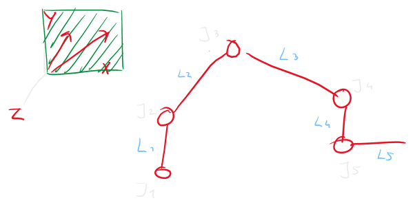
Side Plane View

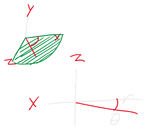
Top Plane View

Joint Layout

The joint chain splits into main positioning links and the wrist:

  J1 (Base Yaw) ──► J2 (Shoulder Pitch) ──► J3 (Elbow Pitch) ──► J4 (Wrist Pitch) ──► J5 (Wrist Roll)
  └───────────── Position Control (X, Y, Z) ────────────────┘ └── Orientation Control (Pitch, Roll) ──┘

Link Lengths:

• $L_1$: Height from the ground ($J_1$) up to the shoulder ($J_2$).
• $L_2$: Upper arm length from shoulder ($J_2$) to elbow ($J_3$).
• $L_3$: Forearm length from elbow ($J_3$) to wrist pitch ($J_4$).
• $L_4$: Wrist bracket length from wrist pitch ($J_4$) to wrist roll ($J_5$).
• $L_5$: Gripper offset from wrist roll ($J_5$) to the tip ($G$).

Pitch Before Roll

Putting pitch first and roll second with intersecting axes at the wrist decouples movement from pointing, letting the math solve neatly across two flat 2D planes.

Step A: Base Angle ($\theta_1$)

Given target coordinates $(X, Y, Z)$ and desired gripper pitch $\alpha_5$, look down at the flat horizontal $XZ$ floor plane to find the base angle $\theta_1$ and horizontal reach $r$:

$\theta_1 = \operatorname{atan2}(Z, X)$

$r = \sqrt{X^2 + Z^2}$

Quadrant Check

Always use atan2(Z, X) in code to handle positive and negative quadrants correctly across a full $360^\circ$ turn.

Step B: Wrist Center ($J_4$)

1. Wrist Pitch Offset ($\alpha_4$): $\alpha_4 = \alpha_5 - 90^\circ$

2. Roll Joint $J_5$ Coordinates: $r_5 = r - L_5 \cos(\alpha_5)$ $y_5 = Y - L_5 \sin(\alpha_5)$

3. Wrist Center $J_4$ Coordinates (relative to shoulder $J_2$ at $r_2 = 0, y_2 = L_1$): $r_4 = r - L_5 \cos(\alpha_5) - L_4 \cos(\alpha_4)$ $y_4 = Y - L_5 \sin(\alpha_5) - L_4 \sin(\alpha_4)$

(When $L_4$ is vertical and $L_5$ is horizontal, this simplifies to $r_4 = r - L_5$ and $y_4 = Y + L_4$).

Step C: Elbow Angle ($\theta_3$)

Looking at the vertical side plane, links $L_2$ and $L_3$ make a triangle between the shoulder ($J_2$), elbow ($J_3$), and wrist center ($J_4$).

        J3 (Elbow)
       /  \
  L2  /    \  L3
     /      \
   J2 ─────── J4 (Wrist Center)
         D

1. Distances from $J_2$ to $J_4$: $\Delta r = r_4 - r_2 = r_4$ $\Delta y = y_4 - y_2 = y_4 - L_1$

2. Direct Distance Squared ($D^2$): $D^2 = (\Delta r)^2 + (\Delta y)^2$

3. Inside Elbow Angle $\alpha_3$ (Law of Cosines): $\alpha_3 = \arccos\left(\frac{L_2^2 + L_3^2 - D^2}{2 \cdot L_2 \cdot L_3}\right)$

4. Motor Angle $\theta_3$: $\theta_3 = \pi - \alpha_3$

Step D: Shoulder Angle ($\theta_2$)

1. Elevation Angle ($\gamma$) to Wrist Center: $\gamma = \operatorname{atan2}(\Delta y, \Delta r)$

2. Inside Triangle Angle $\alpha_2$ (Law of Cosines): $\alpha_2 = \arccos\left(\frac{L_2^2 + D^2 - L_3^2}{2 \cdot L_2 \cdot D}\right)$

3. Shoulder Angle $\theta_2$ (relative to vertical): $\theta_2 = 90^\circ - (\gamma + \alpha_2)$

Step E: Wrist Pitch ($\theta_4$)

Joint $J_4$ compensates for the earlier joint angles to keep the gripper pointed at angle $\alpha_4$:

1. Combined Arm Angle ($\beta_4$): $\beta_4 = 90^\circ - \theta_2 - \theta_3$

2. Wrist Pitch Angle ($\theta_4$): $\theta_4 = \beta_4 - \alpha_4 = 90^\circ - \theta_2 - \theta_3 - \alpha_4$

Elbow-Up vs. Elbow-Down

Because $\arccos$ has both positive and negative roots ($\pm \alpha_2$), the arm has two valid geometric shapes: Elbow-Up and Elbow-Down.

Arm code usually defaults to positive roots for the Elbow-Up stance. Invert the angle sign to use Elbow-Down instead.

---

6. Transformation Matrices

While 2D geometric sketches work well for simple arms, Transformation Matrices are standard for writing out clean, repeatable math on multi-axis arms.

Why Matrices Help:

• Consistent Bookkeeping: Instead of drawing out complex 3D triangles, matrices use standard rules (like Denavit-Hartenberg notation) that apply to every link the same way.
• Unified Math: A single $4 \times 4$ matrix tracks both 3D rotation and linear translation at once, preventing confusing sign mix-ups: $T = \begin{bmatrix} R_{3 \times 3} & \mathbf{p}_{3 \times 1} \\ \mathbf{0}_{1 \times 3} & 1 \end{bmatrix}$
• Simple Chaining: Finding where the tool ends up is just multiplying joint matrices together in order: $T_{\text{base}}^{\text{tool}} = T_0^1 \cdot T_1^2 \cdot T_2^3 \cdot T_3^4 \cdot T_4^5$ If a calculation breaks, you can check each joint matrix one-by-one to find the mistake quickly.

Recommended Resources

Helpful tutorials and books on transformation matrices:

• Video: Inverse Kinematics of Robots (Robotics 101)[cite: 1]
• Book 1: Clemson University: Inverse Kinematics
• Book 2: Introduction to Robotics: Mechanics and Control (Craig)

---

3. Statics & Stability

1. Equilibrium Basics

Statics checks link stiffness, frame bending, and holding motor torque when the robot is standing still:

$\sum \mathbf{F} = \mathbf{0}, \quad \mathbf{a} = \mathbf{0}$

$\sum \boldsymbol{\tau} = \mathbf{0}, \quad \boldsymbol{\alpha} = \mathbf{0}$

Field	Main Question	Forces Included?	Motion Present?	Key Variables
Kinematics	"How is it moving?"	No	Yes	Position, Velocity, Acceleration, Time
Statics	"What keeps it balanced?"	Yes	No	Force, Mass, Torque
Dynamics	"Why is it moving like this?"	Yes	Yes	Force, Mass, Torque, Velocity, Acceleration

1.1 Vectors & Units

Forces and torques point in specific directions in space:

$\mathbf{F} = F_x \hat{\mathbf{i}} + F_y \hat{\mathbf{j}} + F_z \hat{\mathbf{k}}$

Force is measured in Newtons ($1\text{ N} = 1\text{ kg} \cdot 1\text{ m/s}^2$). Under standard Earth gravity ($g = 9.81\text{ m/s}^2$), $1\text{ N}$ is roughly the downward weight of a $102\text{ g}$ apple sitting in your hand.

---

2. Force Decomposition

2.1 Mechanical States

                      +-----------------------------+
                      | System Mechanical States    |
                      +--------------+--------------+
                                     |
         +---------------------------+---------------------------+
         |                                                       |
+--------v--------+                                     +--------v--------+
|  Net Force = 0  |                                     | Net Force != 0  |
|  (Equilibrium)  |                                     |  (Unbalanced)   |
+--------+--------+                                     +--------+--------+
         |                                                       |
   +-----+-----+                                           +-----v-----+
   |           |                                           | Accel > 0 |
+--v--+     +--v--+                                        +-----------+
| v=0 |     | v>0 |
+-----+     +-----+
Static      Dynamic
Equil.      Equil.

Treating an accelerating arm as if it were standing still leads to stalled motors. Moving arms require extra dynamic torque to get up to speed:

$\boldsymbol{\tau}_{\text{peak}} = \boldsymbol{\tau}_{\text{static}} + \mathbf{I} \cdot \boldsymbol{\alpha}$

Sizing motors only for holding torque ($\boldsymbol{\tau}_{\text{static}}$) causes arm lag, structural shaking, and blown motor drivers during sudden accelerations.

2.2 Normal Forces

When a contact surface tilts at an angle $\theta$, the pressing force (normal force) decreases:

$N = m \cdot g \cdot \cos\theta$

Any force $\mathbf{F}$ hitting an arm at angle $\theta$ splits into two perpendicular parts:

$F_x = F \cdot \cos\theta, \quad F_y = F \cdot \sin\theta$

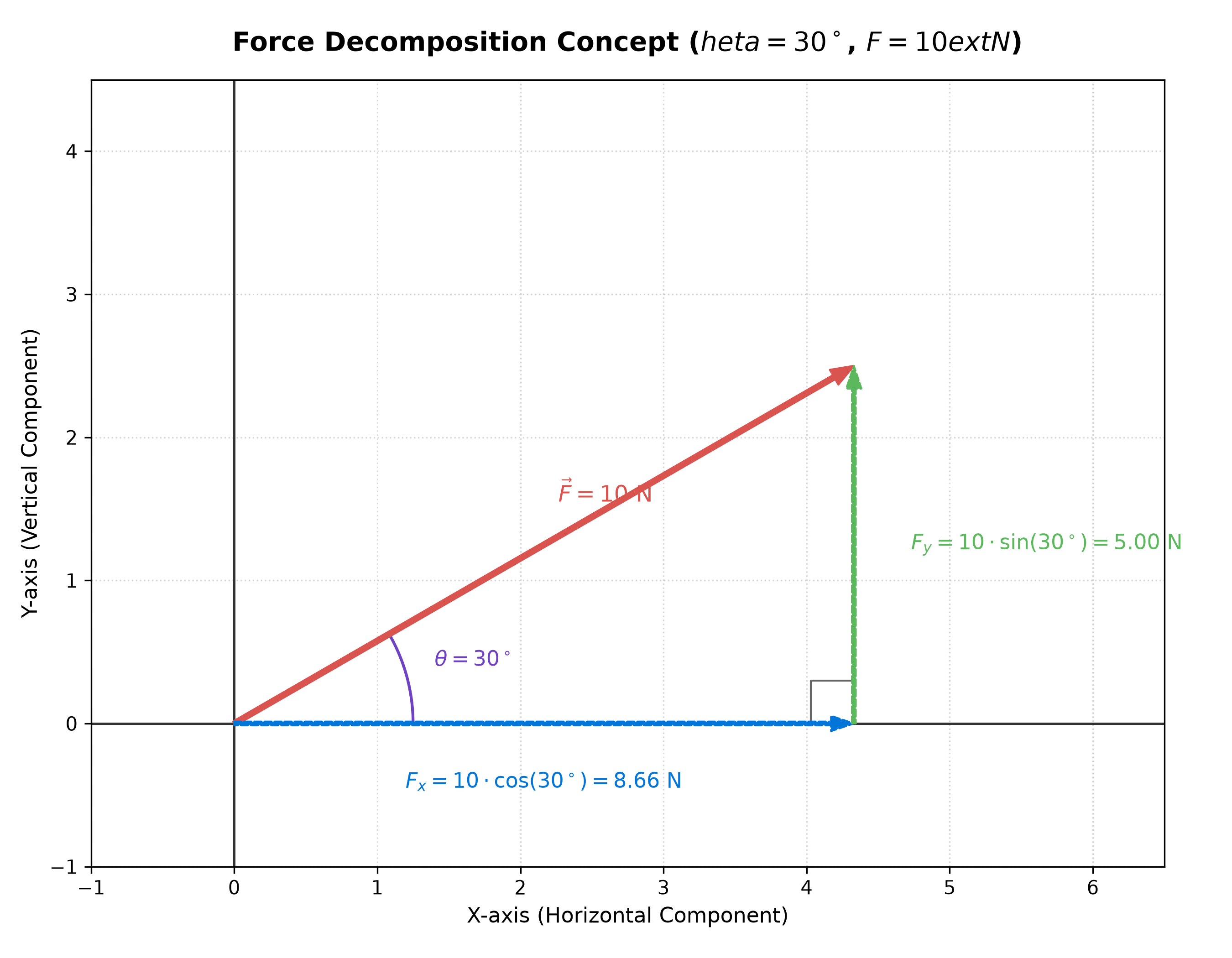
Force Decomposition ($\theta = 30^\circ$)

Example: A $10\text{ N}$ load acting at $\theta = 30^\circ$ splits into:

• $F_x = 10\text{ N} \cdot \cos(30^\circ) = 8.66\text{ N}$
• $F_y = 10\text{ N} \cdot \sin(30^\circ) = 5.00\text{ N}$
• $F = \sqrt{F_x^2 + F_y^2} = \sqrt{(8.66)^2 + (5.00)^2} = 10\text{ N}$

---

3. Gripper Friction

3.1 Friction Model

Static friction ($F_f$) keeps parts from slipping out of the gripper jaws:

$F_f \le \mu \cdot N$

Contact Material	Friction Coeff. ($\mu$)	Design Impact
Rubber Pads	$0.6 - 0.8$	High grip; requires less motor clamping force and draws less current.
Smooth Hard Plastic	$0.25 - 0.4$	Slippery; requires high pinch force, heating up motor windings.

3.2 Parallel Clamping

To support block weight $W = m \cdot g$ vertically across two symmetric jaw pads:

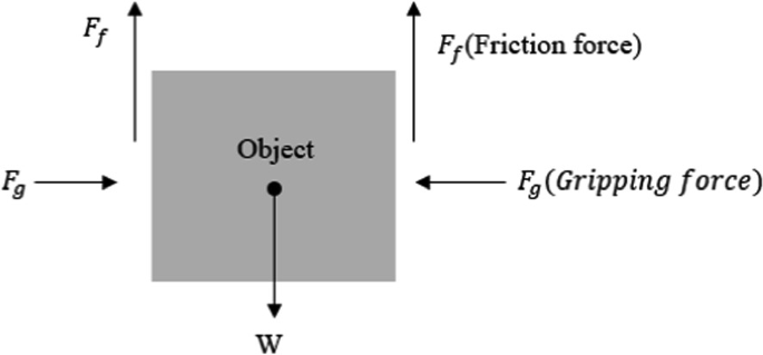
Parallel Clamping Free Body Diagram

$2 \cdot F_f \ge m \cdot g \implies N \ge \frac{m \cdot g}{2\mu}$

The factor of 2 accounts for both jaw pads each taking half of the gravitational load. Gear reduction helps compact motors build this clamping force:

$\tau_{\text{output}} = \tau_{\text{motor}} \cdot N_{\text{gear}} \cdot \eta$

• Parallel Grippers: Linear sliding keeps jaw faces parallel, spreading pinch pressure evenly across the block.
• Hinged Grippers: Jaws pivot along an arc, pinching at odd angles and concentrating pressure on single edges as block sizes change.

---

4. Torque Mechanics

4.1 Lever Arms

Torque is the rotational twist created by a force acting at a distance from a pivot:

$\tau = F \cdot d \cdot \sin\theta$

Torque peaks when pushing at a right angle ($\theta = 90^\circ \implies \tau = F \cdot d$).

Joint Pivot (Tau)                     Link (Length d)                  Payload (F = m*g)
      (O)=================================================================> [ Mass ]
       |                                                                      |
       |<---------------------------- Moment Arm (d) ------------------------>|
       |                                                                      v
   Tau = F * d

4.2 Mechanical Advantage

Joint designs balance speed against holding strength:

• Short Lever (Direct Drive): Attaching a motor right at the joint ($d$ is small) needs high motor torque to hold weight, but gives fast end-effector swing speeds.
• Long Lever (Linkage Drive): Attaching pushrods further out gives mechanical advantage, reducing motor holding torque at the cost of swing speed.

4.3 Servo Heating

Holding torque peaks when the arm reaches straight out horizontally ($\theta = 90^\circ$) and drops to nearly zero when hanging straight down ($d \to 0$).

Thermal Protection Rule

RC servos use internal DC motors. Holding heavy loads in one spot pushes continuous current through the windings, generating heat ($P_{\text{loss}} = I_a^2 R$). Keep continuous holding loads below 50% of rated stall torque:

$\tau_{\text{continuous}} < 0.50 \cdot \tau_{\text{stall}}$

---

5. Base Stability

Weights sticking out from the arm act as tipping levers around the outer support feet.

                       [ Joint 3 / Link ] ---> Force F_links @ d_joint
                            |
                            |   Arm Reach (d_load = 0.4 m)
============================+=======================================> [ Payload 0.3 kg ]
|                                                                        |
| Base Mass Force (F_B)                                                  v
| Center                                                      Payload Weight Force (F_payload)
+-----------------------+
|     Robot Base        |
+-----------------------+
|<- Leg Length Radius ->| 
(P_pivot)               (Trailing Edge)
 Tipping Edge            N_3 (rear) -> 0

5.1 Balance Formula

Typical competition setup numbers:

• Payload Force ($F_{\text{payload}}$): $0.30\text{ kg} \times 9.81\text{ m/s}^2 = 2.943\text{ N}$ at reach $d_{\text{load}} = 0.40\text{ m}$.
• Arm Weight Force ($F_{\text{links}}$): $0.823\text{ N}$ acting at center-of-mass $d_{\text{joint}} = 0.392\text{ m}$.
• Base Downward Weight ($F_B$): $1.02\text{ kg} \times 9.81\text{ m/s}^2 = 10.0\text{ N}$.

The arm starts to tip right when the rear feet lift off the table ($N_{\text{rear}} \to 0$):

$\sum M_P = 0 \implies \tau_{\text{overturn}} - \tau_{\text{restoring}} = 0$

$(F_{\text{payload}} \cdot d_{\text{load}}) + (F_{\text{links}} \cdot d_{\text{joint}}) - (F_B \cdot L) = 0$

$L \ge \frac{(2.943\text{ N} \times 0.40\text{ m}) + (0.823\text{ N} \times 0.392\text{ m})}{10.0\text{ N}} = \frac{1.1772 + 0.3226}{10.0} = 0.15\text{ m} = 15\text{ cm}$

A round base plate with radius $L = 15\text{ cm}$ prevents tipping in all directions and fits inside a $300\text{ mm}$ competition footprint.

5.2 Tripod Bases

Top-Down View of Base Support Geometries:

       Circular Support Base                         3-Leg Tripod Support Base
             .---.                                         Leg 1 (0 deg, Reaction N_1)
           /       \                                             (o)
          |    +    |  Effective Radius                         / | \
           \       /   is L in ALL                             /  |  \   Weak Vector Tipping Line
             '---'     directions                             /   |   \  Distance = L * cos(60 deg)
                       Radius = L                            /    +    \          = 0.5 * L
                                                            /           \
                                                           (o)-----------(o)
                                             Leg 2 (N_2)                   Leg 3 (N_3 -> 0)
                                                              Tipping Axis (N_3 = 0)

On a 3-legged tripod base, the shortest distance from the center to a tipping line lies directly between two legs:

$d_{\text{eff}} = L \cdot \cos(60^\circ) = 0.50 \cdot L$

To keep the real support distance at $d_{\text{eff}} \ge 15\text{ cm}$ in this weak direction, make the legs longer:

$L_{\text{tripod}} \ge \frac{L_{\text{calculated}}}{\cos(60^\circ)} = \frac{15\text{ cm}}{0.50} = 30\text{ cm}$

A tripod base needs $30\text{ cm}$ long legs to avoid tipping, or the base should switch to 4 legs or a flat round plate.

---

4. Dynamics

1. Motion Derivatives

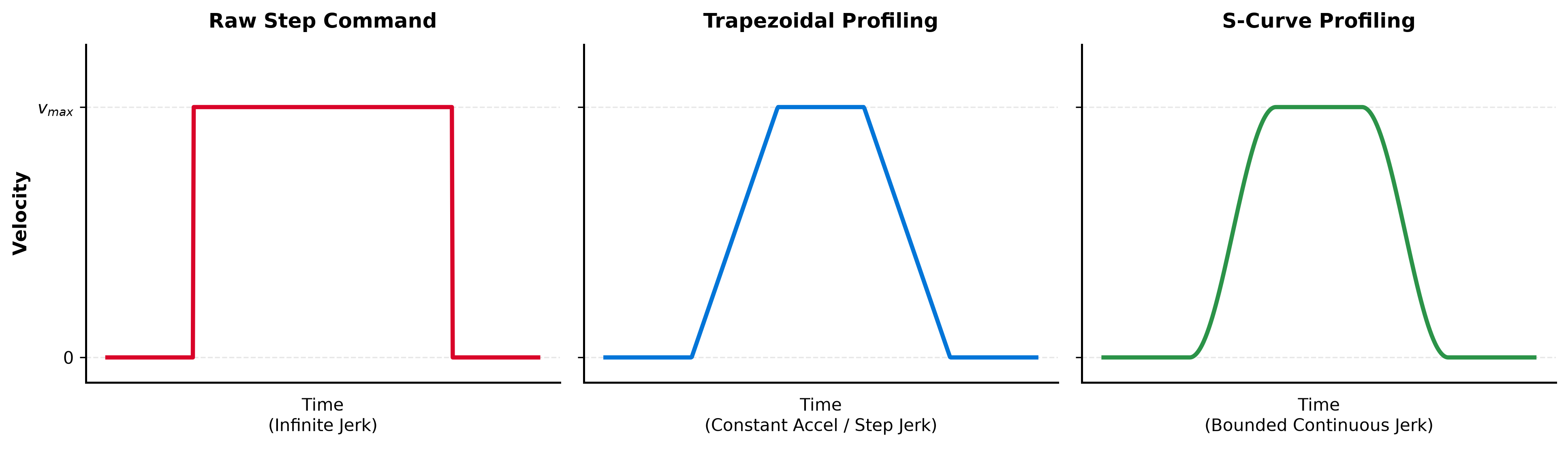
Rapid speed changes create inertial forces ($\mathbf{F} = m \mathbf{a}$). Sudden raw motor steps cause transient accelerations from $6\text{ to }15\text{ m/s}^2$ ($0.6\text{ to }1.5 \times g$), shocking gear teeth.

Jerk ($j$) tracks how fast that force hits:

$j = \frac{da}{dt} = \frac{d^3x}{dt^3} \quad \left[\text{m/s}^3\right], \quad \frac{d\mathbf{F}}{dt} = m \cdot j$

• Unfiltered Motor Steps: $300\text{ to }600\text{ m/s}^3$ (instant impact spike).
• Smooth Transport Limit: $\approx 50\text{ m/s}^3$ (steady human launch).

Jerk does not change the average or nominal force on a system. It dictates how rapidly that force hits. Because real-world materials have elasticity, flex, and inertia, applying force nearly instantaneously causes shock-loading, creating severe peak-force spikes for a brief moment even though the average force remains identical. Because modeling these transient material vibrations in code is rarely practical, standard engineering practice relies on software trajectory smoothing (like S-curves) to minimize jerk, paired with safety factors (1.5× to 2.5×) based on the amount of jerk in the system.

• Trapezoidal Profile: Caps top speed and acceleration, but sharp profile corners still cause quick jerk spikes.
• S-Curve Profile (7-Segment): Uses smooth acceleration ramps ($\frac{da}{dt} \le j_{\max}$), removing shock loads and stopping the arm from shaking.

---

2. Parasitic Forces

Scenario 1: Vertical Lift

Extending the pinch-force formula from Section 3.3 to include upward lift acceleration ($a_y$):

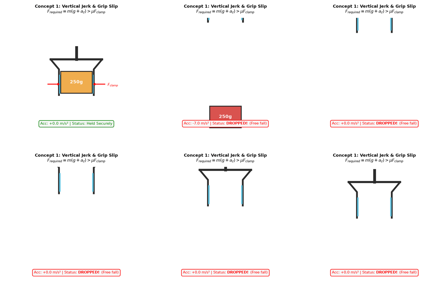
Vertical Slip Demonstration

$2 \mu N \ge m(g + a_y)$

For a $0.25\text{ kg}$ block lifted at $a_y = 1.0 \times g = 9.81\text{ m/s}^2$:

• Holding Force: $F_{\text{static}} = 0.25 \times 9.81 = 2.45\text{ N}$
• Lifting Force: $F_{\text{dynamic}} = 0.25 \times (9.81 + 9.81) = 4.90\text{ N} \quad (2\times \text{ static})$

Clamping sized only for static resting weight will drop the block as soon as the arm jerks upward.

Scenario 2: Stopping Momentum

Slamming the brakes on a forward reach throws weight forward at reach $L$:

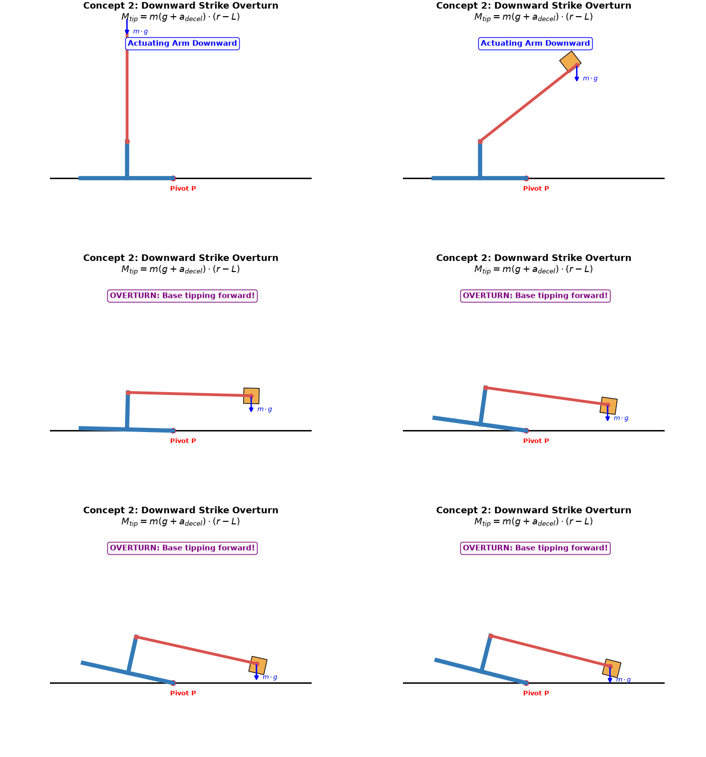
Dynamic Tipping

Stopping forces reaching $\approx 5\text{ N}$ act across length $L$, creating up to $3\times$ the resting tipping torque on the base and shoulder motor.

Scenario 3: Base Swivel

Fast rotations around the base ($\theta_1$) create sideways and outward forces:

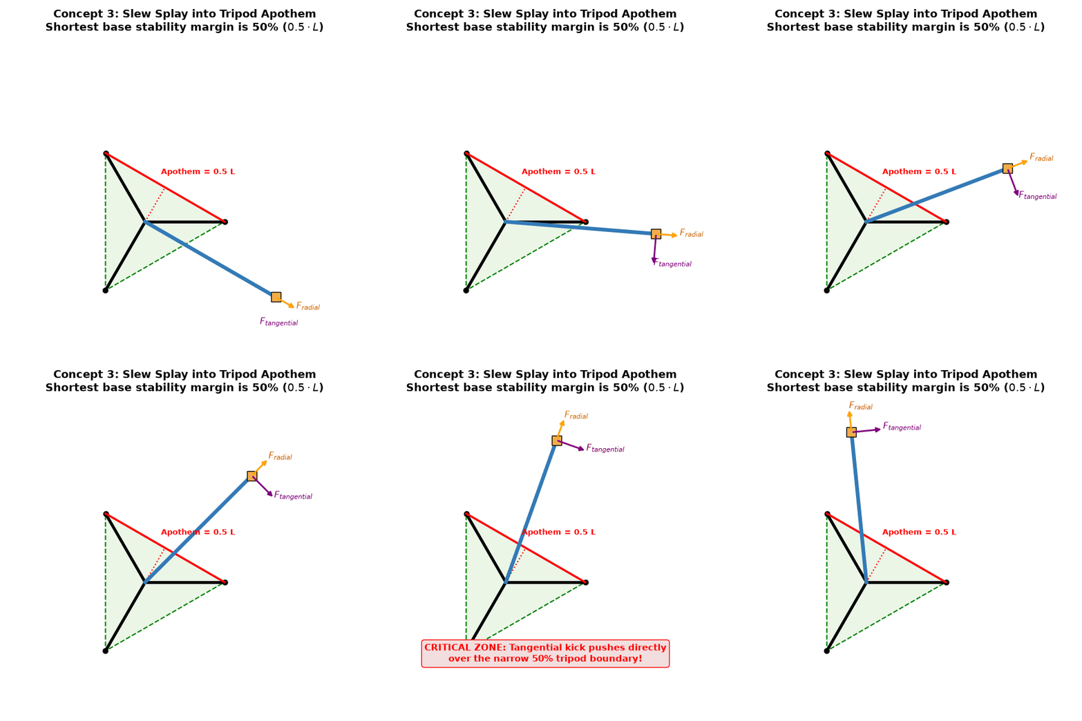
Base Swivel

• Outward Force: $F_{\text{centrifugal}} = m \cdot \omega^2 \cdot L \sim 1\text{ N}$ ($\approx \frac{1}{3}\times$ block weight).
• Sideways Force: $F_{\text{tangential}} = m \cdot \alpha \cdot L \sim 3\text{ N}$ ($\approx 1\times$ block weight).

These forces twist motor shafts and bend thin 3D-printed links sideways.

Scenario	Main Cause	Force Impact	Critical Risk
1. Upward Lift	Lift acceleration ($a_y$), downward inertia ($m a_y$)	$2\times$ required grip force ($N$)	Dropping blocks during lift
2. Stopping Reach	Braking ($-a$), tipping lever ($\tau = F_{\text{dyn}} L$)	Forces reach $\approx 5\text{ N}$ ($3\times$ base torque)	Tipping base, stalled shoulder
3. Base Turn ($\theta_1$)	Outward pull ($F_c$), sideways push ($F_t$)	Outward: $\sim 1\text{ N}$ Sideways: $\sim 3\text{ N}$	Bent arm links, twisted motor shafts

---

3. Engineering Rules

Full dynamic arm equations require solving coupled matrix math:

$\mathbf{M}(\boldsymbol{\theta})\boldsymbol{\ddot{\theta}} + \mathbf{C}(\boldsymbol{\theta}, \boldsymbol{\dot{\theta}})\boldsymbol{\dot{\theta}} + \mathbf{G}(\boldsymbol{\theta}) = \boldsymbol{\tau}$

Small microcontrollers cannot compute these matrices in real time. Instead, engineers follow a practical 3-step design approach:

+-------------------------------------------------------------------+
| STEP 1: Vector Estimation                                         |
| Estimate worst-case forces at full arm reach and top speed.       |
+-------------------------------------------------------------------+
                                  |
                                  v
+-------------------------------------------------------------------+
| STEP 2: Smooth Profiles                                           |
| Use S-curve ramps in software to stop sudden jerk and spikes.     |
+-------------------------------------------------------------------+
                                  |
                                  v
+-------------------------------------------------------------------+
| STEP 3: Safety Factors                                            |
| Multiply holding torque by 1.5x - 2.5x to size parts safely.      |
+-------------------------------------------------------------------+

1. Vector Estimation: Check peak forces when the arm is stretched out with a full $250\text{ g}$ block.
2. Smooth Profiles: Add acceleration ramps in firmware to eliminate jerky force spikes.
3. Safety Factors: Multiply holding torque by $1.5\text{ to }2.5\times$ to pick strong enough motors without needing real-time matrix math.

---

5. Arm Architectures

1. Main Layouts

Robotic arms generally fall into three kinematic styles:

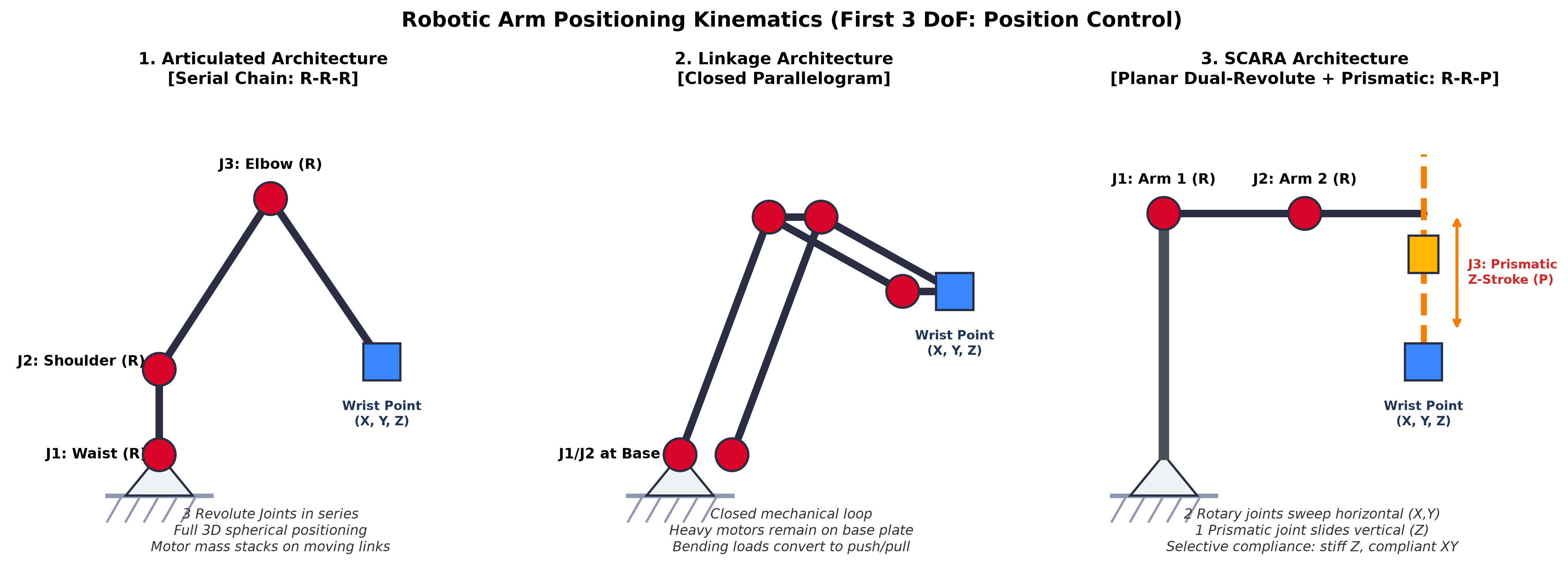
1.1 Articulated Arms

An articulated arm connects rotary joints in a row, like a human arm. It divides motion into two main sections:

• Position (First 3 DoF): 3 rotary joints (waist turn, shoulder tilt, and elbow tilt) move the wrist center across 3D space $(X, Y, Z)$.
• Orientation (Last 3 DoF): The wrist rotates the tool (Roll, Pitch, Yaw).

Base / Shoulder / Elbow Joints (3 DoF) ──► Position Control (X, Y, Z Translation)
Wrist Assembly (3 DoF)                 ──► Orientation Control (Roll, Pitch, Yaw)

Meeting all wrist axes at a single point (spherical wrist) keeps orientation changes from moving the arm tip:

• Pitch: Tilting up and down.
• Yaw: Turning side to side.
• Roll: Twisting along the tool axis.

This keeps positioning math $(X, Y, Z)$ completely separate from pointing math (Roll, Pitch, Yaw).

1.2 Linkage Arms

A linkage arm uses parallel bars to form a closed parallelogram loop.

Instead of each motor having to carry the weight of all downstream motors:

• Bending forces turn into simple push and pull forces along the parallel bars.
• Heavy joint motors can sit directly on the sturdy base plate rather than riding along the moving links.
• Keeping heavy motors on the base makes the moving arm lighter, reducing strain.

1.3 SCARA Arms

A SCARA arm combines two horizontal rotary joints with one vertical linear slider:

• Two Rotary Joints: Move parallel to the table to sweep across the horizontal $(X, Y)$ plane.
• One Linear Slider: Moves straight up and down along the vertical $Z$-axis.

This layout gives selective stiffness: the arm is very rigid vertically to push parts into place, but stays compliant horizontally to guide blocks into position smoothly.

1.4 Joint Summary

As established in Section 2.2, arms combine standard joint types:

• Prismatic (1 DoF, Linear): Slides on a straight rail; stiff and simple (used in 3D printers and CNCs).
• Revolute (1 DoF, Rotary): Spins around a pin (the basic building block of robot arms).
• Universal (2 DoF, Rotary): Bends across two perpendicular hinges (used in drive shafts).
• Cylindrical (2 DoF, Slider & Spinner): Slides and turns on one shaft (found in drill presses).
• Spherical (3 DoF, Rotary): Ball-and-socket pivot (used in camera mounts and wrist assemblies).

---

2. Workspace Reach

2.1 Starting Size

Competition rules require the robot to fit into a $300 \times 450\text{ mm}$ starting footprint. Reaching distant scoring zones ($175 \times 175\text{ mm}$) requires an arm that folds tightly:

START BOUNDING BOX ENVELOPE (300 mm x 450 mm Base Boundary)
+-------------------------------------------------------------+
|  Folded Storage Configuration (Pre-Match State)             |
|                                                             |
|       (θ2 Fold Angle)                                       |
|         \  Link 2                                           |
|          \                                                  |
|   Base ([O])======Link 1=====>                              |
|       (θ1 Joint Angle)                                      |
|                                                             |
|  * High link folding angles (θ1, θ2) maintain               |
|    full enclosure within 300 mm x 450 mm boundaries.        |
+-------------------------------------------------------------+
                              |
                              | Unfolding / Deployment Sequence
                              v
EXTENDED WORKSPACE ENVELOPE (Active Operational State)
+-------------------------------------------------------------+
| Base ([O])=======Link 1=======>=======Link 2=======> (EE)   |
|                                                             |
|  * Maximum link extension expands reachable radius to       |
|    access distant field objects and 175 mm x 175 mm stacks. |
+-------------------------------------------------------------+

Arms with good folding geometry tuck their links into the box at the start, then extend outward to full reach during the run.

2.2 Reach Profiles

Reachable working areas differ by arm type:

• Articulated Arm: Reaches in a wide dome shape. It can pick up items off the floor, high up, or behind itself with great dexterity.
• Linkage Arm: Reaches along a curved vertical slice. Parallel bars limit how high or far behind itself it can reach compared to an open serial arm.
• SCARA Arm: Sweeps out a flat circle or wedge. Its reach is wide horizontally, but vertical travel is limited by the length of its vertical sliding rod.

2.3 Dead Zones

Physical link collisions and mechanical stops create areas the gripper cannot reach:

• Linkage Arm: Has an hourglass-shaped dead zone right around its shoulder pivot because the parallel bars hit each other if drawn too close to the base.
• SCARA Arm: Has a small dead zone around its center pole, but can otherwise work close in as long as links fold beside each other.
• Articulated Arm: Has few dead zones, mostly when reaching straight out at maximum limit or directly above its base swivel.

---

3. Architecture Comparison

3.1 Motor Weight

Where motors are mounted changes how heavy the arm feels during fast moves:

$I_{\text{link}} = \sum_{i=1}^{n} m_i r_i^2$

$\tau_j = I_j \alpha_j + \tau_{\text{gravity}}$

$\tau_{\text{gravity}} = m_i g r_i \cos(\theta_i)$

ARTICULATED ARM (Serial Actuation Pattern):
[Base Frame] ===> (Motor 1) --- Link 1 --- (Motor 2) --- Link 2 --- (Motor 3) --- [End-Effector]
                                            ^                       ^
                                            +-- Cantilevered Mass --+
                                            (High Distal Inertia & Compounded Torque)

LINKAGE ARM (Base-Mounted Actuation Pattern):
[Base Motor 1] --+
                 +===> [Parallel Structural Linkage] ===> [Lightweight End-Effector]
[Base Motor 2] --+
(Stationary Actuator Mass = Minimal Distal Inertia & Reduced Bending Moments)

In an articulated arm, mounting motors out along the links puts heavy mass far from the base, increasing inertia ($I \propto m r^2$) and demanding larger motors to accelerate.

In a linkage arm, mounting motors on the stationary base frame transfers force through light pushrods. This keeps the moving arm light and cuts down on required motor torque.

3.2 Speed & Complexity

• Math Complexity: Articulated arms need inverse kinematics code to solve multi-axis geometry. Intersecting wrist axes keeps this math manageable. SCARA arms use simple flat 2D geometry, making their math very fast to compute.
• Build Tolerances: Articulated and SCARA arms use single pivot pins that are easy to align. Linkage arms have many parallel joints; if hole spacing is off by even a fraction of a millimeter, the bars will jam.

3.3 Trade-Off Table

Criterion	Articulated Arm	Linkage Arm	SCARA Arm
Reach	5/5 (High): Reaches all around in a wide 3D dome, from ground level to high up.	3/5 (Medium): Sweeps along a fixed arc; limited overhead and rear clearance.	2/5 (Low–Mid): Good flat table reach, but vertical travel is strictly tied to slider stroke.
Strength	1/5 (Low): Motor weight out on the links creates high bending strain at full reach.	4/5 (High): Parallel bars turn bending forces into push-pull tension and compression.	3/5 (Medium): Solid vertical slide rail takes down-force well, but links face sideways flex.
Speed	2/5 (Low–Mid): Heavy moving links build high inertia, slowing down quick stops and turns.	3/5 (Medium): Motors sit on the base, keeping moving links light for steady acceleration.	4/5 (High): Built for fast horizontal pick-and-place sweeps across the workspace.
Design Effort	Medium: Needs custom brackets and 3D modeling from scratch for each serial joint.	Medium: Ensuring the links don't hit each other and are sized properly to ensure a good reach.	High: Requires integrating linear sliders, belts, and rotary bearings from the ground up.
Build & Assembly	Easy: Modular rotary joints with single pivot pins that are straightforward to assemble.	Medium: Parallel pin holes must line up cleanly to avoid binding, but parts are pre-dimensioned.	Hard: Linear rails must be aligned precisely straight to prevent the vertical axis from sticking.

---

4. Task Matching

4.1 Block Weights

Game block weight drives how stiff the arm needs to be:

LIGHTWEIGHT PAYLOADS (30 g Cubes / 60 g Blocks)     HEAVY PAYLOADS (250 g Solid Blocks)
- Minimal gravitational torque (τ_gravity)          - Severe static torque (τ = m * g * d)
- Favors open-chain Articulated / SCARA arms        - Favors closed-loop Linkage arms
- Priority: Rapid trajectory acceleration            - Priority: High structural rigidity & low flexure

• Light Blocks ($30\text{ g}$ to $60\text{ g}$): Add very little tipping load ($\tau_{\text{gravity}}$). Articulated or SCARA arms move these quickly without noticeable flex.
• Heavy Blocks ($250\text{ g}$): Create high bending leverage ($\tau = F \cdot d$) at full reach. Linkage arms or rigid SCARA rods handle these heavier loads without drooping.

4.2 Camera Views

Overhead cameras find blocks and send target coordinates to the robot:

{
  "id": 1,
  "x": 420.6,
  "y": -366.6,
  "theta": 314.4
}

How the gripper approaches the block determines whether the camera can track it:

OVERHEAD VISION CAMERA
       |
       v  (Unobstructed Optical Path)
[ ArUco Visual Tag ]
+------------------+
|   Target Block   |
+------------------+
       ^
       | (Lateral Approach)
[ Side-Gripping Mechanism ]  ──► Preserves Visual Tag Line-of-Sight

VS.

   [ Top-Gripping End-Effector ]
               |
               v (Direct Vertical Approach)
[ Physical Occlusion Breaks Camera Tracking Data Stream ]
+------------------+
|   Target Block   |
+------------------+

• Top Grippers: Lowering directly over the block blocks the camera's view of the ArUco marker tag, cutting off position tracking mid-grip.
• Side Grippers: Grabbing from the side leaves the top tag visible, letting the camera verify block position all the way through the stack.

4.3 Motor Choices

Picking motors balances travel range, control accuracy, and packaging size:

• $180^\circ$ RC Servos: Built-in controllers and feedback make them easy to wire and code. However, their limited $180^\circ$ swing limit the range of motion, which is problematic for the base joint.
• Stepper Motors: Spin continuously with precise step control, allowing tight folding to meet starting box size limits. They need homing switches to zero out on boot.
• Serial Bus Servos: Servo variant that are both able to rotate continuously and maintain closed-loop control. While still less accurate than a stepper motor, it is more accurate than a RC servo. It involves significantly more complex software controls to use compared to a RC servo.